Source dataset
The copied data dictionary identifies the source dataset as kaistrain.dta.
This example shows how one study dataset moves from basic checks to statistical tables, figures, and a report draft. The technical steps follow: prepare the dataset, explore it with EDA, build Tables 1 to 3, then generate the AI-assisted manuscript and export package.
Start with the dataset and work forward. Each table, figure, and report section links back to a source output so you can see where it came from, including the dataset checks, statistical results, and export files.
Confirm the source dataset, records, variables, labels, value distributions, and missingness before using the results.
Use the data dictionary, observed distributions, and descriptive checks to understand the data before formal tables.
Describe participant characteristics by sex so the study population is clear before interpreting outcomes.
Estimate HIV prevalence by sex and subgroup, with weighted percentages and confidence intervals.
Review simple and multiple logistic regression estimates for predictors of HIV positivity.
Generate the manuscript-style draft only after the checked source outputs are available for review.
Before any table is treated as meaningful, the user needs to know what dataset was loaded, how many records are present, and what each variable represents.
The copied data dictionary identifies the source dataset as kaistrain.dta.
The example includes 13,614 records and 26 variables in the source data dictionary.
The output keeps field names, labels, formats, missingness, and observed values available before the tables are interpreted.
Start with the data dictionary when reviewing this example, then move to the analysis tables.
Open data dictionary →In this public package, the EDA evidence is mainly visible through the data dictionary and the descriptive distribution outputs. The goal is to catch coding, missingness, and distribution issues before the formal tables are read as final.
The data dictionary shows observed value distributions so a reviewer can see how variables are coded.
Missingness is kept close to the variable descriptions instead of being separated from the analysis trail.
The manuscript package also carries a descriptive distribution figure from the saved frequency output.
The example does not expose a full EDA dashboard. It shows the copied outputs that are available for review now.
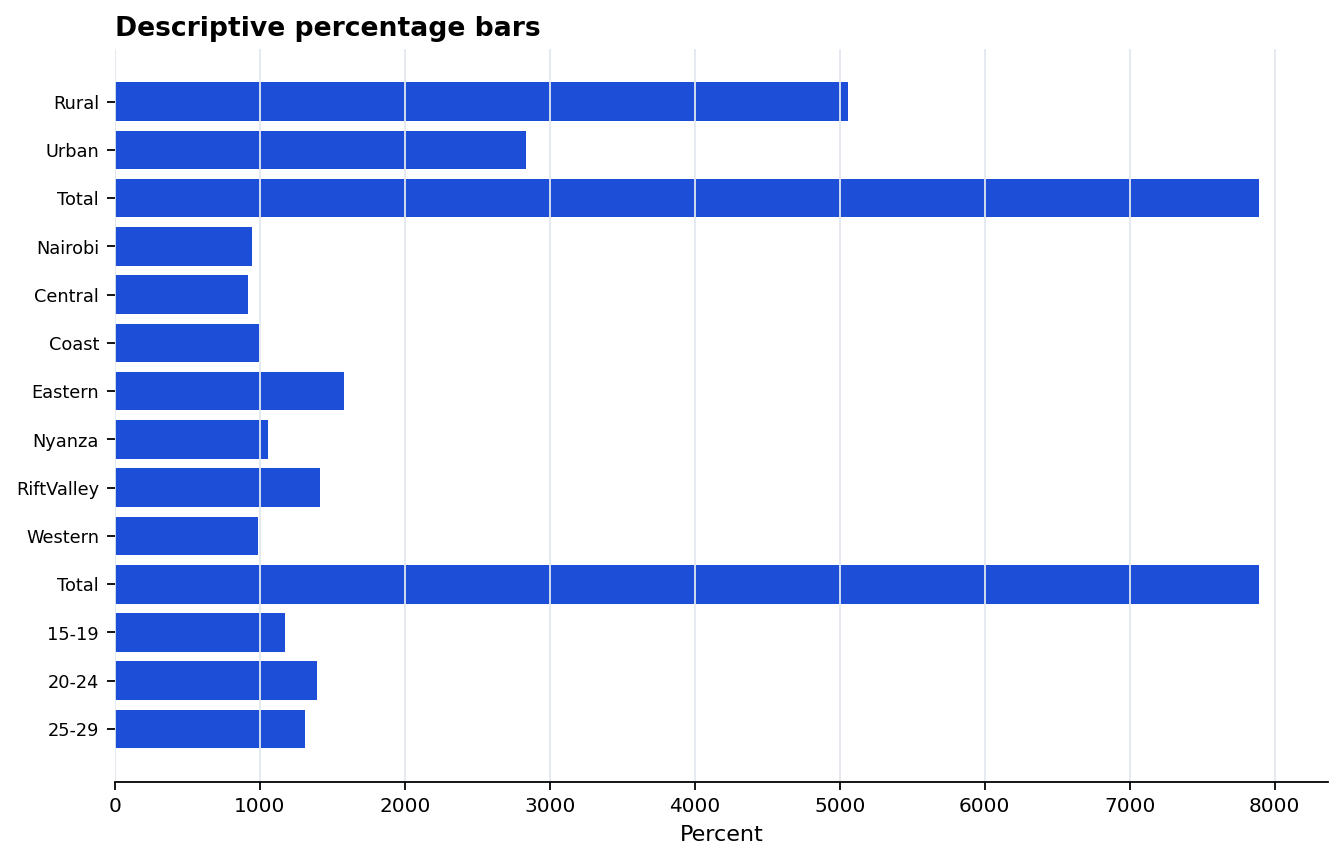
Table 1 helps a reviewer understand the study population before moving to prevalence or predictor results.
Participant characteristics by Sex, with N=13,614.
The output records aiweight, strata2, and qclust for the survey-style table.
The table keeps weighted estimates, confidence intervals, p-values, footnotes, and metadata visible.
Use Table 1 to check participant structure before interpreting Table 2 prevalence results.
Open Table 1 →Table 2 estimates HIV prevalence among study participants by sex and subgroup, with weighted percentages and confidence intervals.
The prevalence output uses hiv = 1 as the outcome-positive definition.
The table reports 648 HIV-positive records among 11,534 analyzable participants for the selected output.
The output records abweight, strata2, and qclust, plus footnotes about approximation and weighting.
Review the full table before relying on the short prevalence summary.
Open Table 2 →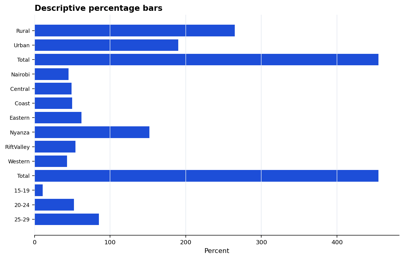
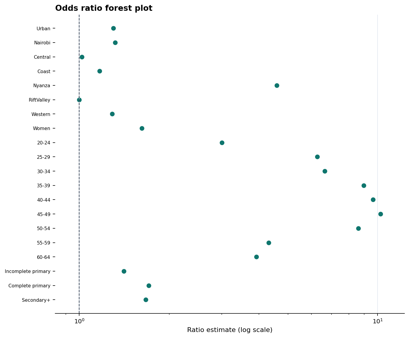
Table 3 shows simple and multiple logistic regression estimates together, so a reviewer can see both unadjusted and adjusted results before reading the manuscript draft.
| Predictor signal | Simple estimate | Adjusted estimate | Review note |
|---|---|---|---|
| Nyanza vs Eastern | OR 4.59 | Adjusted OR 4.69 | Strong regional signal in both simple and multiple outputs. |
| Women vs men | OR 1.62 | Adjusted OR 1.44 | Sex remains visible after adjustment in the copied table. |
| Modeling caveat | Weighted output | Robust-covariance approximation | The table notes that it does not reproduce PROC SURVEYLOGISTIC Taylor variance exactly. |
The AI-assisted manuscript is useful because it pulls the analysis trail into a readable draft. It should still be checked against the data dictionary, Table 1, Table 2, Table 3, and figures before publication or formal use.
The draft covers HIV prevalence and associated factors among adults aged 15-64 in KAIS 2012. It is best read as a reporting workflow example, not as a final journal submission.
Use PDF for review and DOCX when the report needs edits or comments.
Open PDF → Open DOCX →This page stays readable by showing the path and key values. The linked files are the source evidence for anyone who wants to inspect the details.
Data dictionary with labels, formats, observed values, missingness, and source dataset context.
Table 1 characteristics, Table 2 prevalence, and Table 3 predictors are all available as standalone HTML outputs.
The manuscript package carries prevalence, descriptive distribution, and logistic-regression figures.
HTML, PDF, DOCX, and Markdown outputs are kept together for review and reuse.
The example shows the analysis flow and copied outputs. The live app is where users would upload data, run checks, create tables, generate reports, and manage saved jobs.